ECON 730: Causal Inference with Panel Data
Lecture 4: Efficient Estimation for Staggered Rollout Designs
Emory University
Spring 2026
Motivation: Application
Application: Reducing Police Misconduct
- Reducing police misconduct and the use of force is an important policy objective
- Wood, Tyler, and Papachristos (2020) (PNAS): Randomized rollout of procedural justice training for Chicago police officers
- Emphasized respect, neutrality, and transparency in the exercise of authority
- Original study found large and significant reductions in complaints/use of force
- Wood et al. (2020): a re-analysis using Callaway and Sant’Anna (2021)’s full-adjustment approach (\(\beta = 1\)):
- No significant impacts on complaints; borderline effects on use of force; wide CIs
Two natural questions: Is the sampling-based approach to inference adequate? How should we optimally use pre-treatment data when treatment timing is random?
The Precision Problem: Event Study
Re-analysis by Wood et al. (2020) using full baseline adjustment (\(\beta = 1\)):
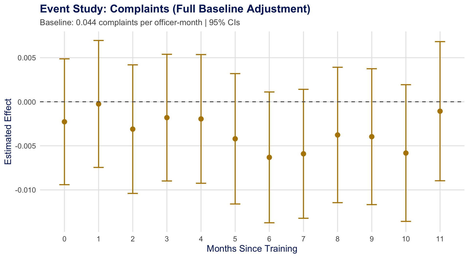
Officers averaged 0.044 complaints/month before training. Estimates suggest \(\approx 11\%\) reduction — but confidence intervals are wide.
The Precision Problem: All Outcomes
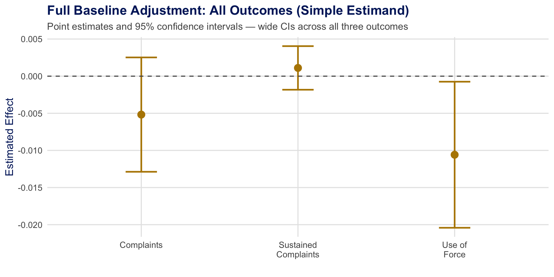
Is this imprecision inherent to the data, or is there a more efficient way to use pre-treatment information?
How should we optimally use pre-treatment data when treatment timing is random?
By finding the efficient adjustment weight.
In Roth et al. (2023), we introduce a design-based framework and derive the efficient estimator for staggered rollout designs.
Preview of Results
- Roth et al. (2023) introduce a design-based framework formalizing random treatment timing
- Consider a large class of causal parameters aggregating effects across periods and cohorts
- Solve for the efficient estimator in a class of pre-treatment adjustment estimators
Key results:
- SE reductions of 2\(\times\) or more in Monte Carlo simulations and applications
- Both \(t\)-based and Fisher Randomization Test inference
- Implemented in the R package
staggered
Roadmap
Framework: Staggered rollout with random treatment timing
Special Case: Two-period model (building intuition)
Causal Parameters: Aggregations of \(ATE(g,t)\)
Class of Estimators: \(\hat{\theta}_\beta = \hat{\theta}_0 - \hat{X}'\beta\)
The Efficient Estimator: \(\beta^*\) and plug-in version
Inference: \(t\)-based CIs and Fisher Randomization Tests
R Implementation: The
staggeredpackageApplication: Police training revisited
From Experiments to Staggered Designs
- Lecture 3: We studied randomized experiments with design-based inference
- Known treatment probabilities \(\to\) unbiased Horvitz-Thompson estimation
- No use of pre-treatment data for efficiency
- This lecture: What if treatment timing is the random variable?
- Staggered rollout: units are treated at different times
- Pre-treatment outcomes are available — should we use them?
The core question: In a randomized experiment, should you adjust for baseline covariates? How much? This is the classical regression adjustment debate (Freedman 2008; Lin 2013). Here, the “covariate” is the pre-treatment outcome.
Framework
Framework
- Finite population: \(N\) units, \(T\) periods (\(i = 1, \ldots, N\); \(t = 1, \ldots, T\))
- Treatment timing: Unit \(i\) first treated at \(G_i \in \mathcal{G} \subset \{1, \ldots, T\} \cup \{\infty\}\)
- \(G_i = \infty\): never treated. Treatment is absorbing (no switching on/off)
- Potential outcomes: \(Y_{i,t}(g)\) = outcome for unit \(i\) in period \(t\) if first treated at \(g\)
- Observed outcomes: \(Y_{i,t} = \sum_{g} \mathbf{1}[G_i = g]\, Y_{i,t}(g)\)
Design-based framework: Potential outcomes \(Y_{i,t}(\cdot)\) and cohort sizes \(N_g = \sum_i \mathbf{1}[G_i = g]\) are fixed; only the treatment assignment \(G\) is stochastic.
Connection to Lecture 2: Same \(Y_{i,t}(g)\) notation. Connection to Lecture 3: Same design-based perspective, but now with absorbing staggered treatment.
Design-Based Uncertainty
Randomization Inference: potential outcomes are fixed; only treatment timing \(G\) is permuted
Actual Sample
| Unit | \(Y(2)\) | \(Y(3)\) | \(Y(4)\) | \(G_i\) |
|---|---|---|---|---|
| 1 | ? | ? | \(\checkmark\) | 4 |
| 2 | \(\checkmark\) | ? | ? | 2 |
| 3 | ? | ? | \(\checkmark\) | 4 |
| 4 | ? | \(\checkmark\) | ? | 3 |
| \(N\) | \(\checkmark\) | ? | ? | 2 |
Alternative I
| Unit | \(Y(2)\) | \(Y(3)\) | \(Y(4)\) | \(G_i\) |
|---|---|---|---|---|
| 1 | ? | \(\checkmark\) | ? | 3 |
| 2 | ? | \(\checkmark\) | ? | 3 |
| 3 | ? | ? | \(\checkmark\) | 4 |
| 4 | \(\checkmark\) | ? | ? | 2 |
| \(N\) | \(\checkmark\) | ? | ? | 2 |
Alternative II
| Unit | \(Y(2)\) | \(Y(3)\) | \(Y(4)\) | \(G_i\) |
|---|---|---|---|---|
| 1 | ? | ? | \(\checkmark\) | 4 |
| 2 | ? | \(\checkmark\) | ? | 3 |
| 3 | \(\checkmark\) | ? | ? | 2 |
| 4 | ? | ? | \(\checkmark\) | 4 |
| \(N\) | ? | ? | \(\checkmark\) | 3 |
Potential outcomes are the same across samples. Only \(G_i\) (and hence which POs we observe) changes.
Assumption 1: Random Treatment Timing
Assumption (Random Treatment Timing). Let \(G = (G_1, \ldots, G_N)\). Then:
\[\Pr(G = \tilde{g}) = \frac{\prod_{g \in \mathcal{G}} N_g!}{N!} \quad \text{if } \sum_i \mathbf{1}[\tilde{g}_i = g] = N_g \text{ for all } g, \text{ and zero otherwise.}\]
- Interpretation: Any permutation of treatment timing preserving cohort sizes is equally likely
- Examples of plausible random timing:
- By design: randomized rollout of police training (Wood, Tyler, and Papachristos 2020)
- Quasi-random: timing of parental deaths (Druedahl and Martinello 2022), health shocks (Fadlon and Nielsen 2021), office closings (Deshpande and Li 2019), stimulus payments (Parker et al. 2013)
Assumption 2: No Anticipation
Assumption (No Anticipation). For all units \(i\), periods \(t\), and treatment dates \(g, g' > t\):
\[Y_{i,t}(g) = Y_{i,t}(g')\]
- Interpretation: Outcomes before treatment do not depend on when treatment will start
- Connection to Lecture 3: Same no-anticipation assumption. Under this assumption, we write \(Y_{i,t}(\infty)\) for the “untreated” potential outcome
- Caveat: May fail if treatment timing is announced in advance (Malani and Reif 2015)
Assessing Random Treatment Timing
- Random treatment timing is a strong assumption — how can we assess its plausibility?
- Key idea: Under random treatment timing + no anticipation, pre-treatment outcomes should be balanced across cohorts (just like covariate balance in RCTs!)
- Roth et al. (2023) propose pre-tests to assess plausibility of random treatment timing
- Balance checks implemented in R package
staggered
- Balance checks implemented in R package
- If random treatment timing fails, weaker assumptions (covered in later lectures) can still justify causal inference — but without the efficiency gains derived here
Bottom line: Random treatment timing provides additional structure beyond basic unconfoundedness. When plausible, it enables more efficient estimation. Balance checks help assess its credibility.
Special Case: Two-Period Model
Two-Period Model: Building Intuition
- Setup: \(T = 2\), \(\mathcal{G} = \{2, \infty\}\). Some units treated in period 2, rest never treated.
- Under randomization + no anticipation, this is analogous to a cross-sectional randomized experiment:
| Outcome: \(Y_i = Y_{i,t{=}2}\) | (post-treatment outcome) |
| Covariate: \(X_i = Y_{i,t{=}1} \equiv Y_{i,t{=}1}(\infty)\) | (pre-treatment outcome) |
| Treatment: \(D_i = \mathbf{1}[G_i = 2]\) | (treatment indicator) |
We use the two-period case as a running example to build intuition before moving to the general staggered case.
Two-Period: Target Parameter and Estimator Class
Target: \(\theta = \frac{1}{N} \sum_{i=1}^{N} [Y_{i,2}(2) - Y_{i,2}(\infty)]\) \(\qquad\) Class of estimators: \[\hat{\theta}_\beta = \underbrace{(\bar{Y}_{22} - \bar{Y}_{2\infty})}_{\text{Post-treatment diff}} - \beta \underbrace{(\bar{Y}_{12} - \bar{Y}_{1\infty})}_{\text{Pre-treatment diff}}\]
where \(\bar{Y}_{sg} = N_g^{-1} \sum_{i:\, G_i = g} Y_{i,s}\) is the period-\(s\) sample mean for cohort \(g\), and \(\beta \in \mathbb{R}\).
| \(\beta = 0\): | No adjustment (difference-in-means) | ignores pre-treatment data |
| \(\beta = 1\): | Full baseline adjustment | subtracts entire pre-treatment diff |
| \(\beta \in (0,1)\): | Partial adjustment | intermediate correction |
| \(\beta < 0\) or \(\beta > 1\): | Extrapolation | also allowed; optimal \(\beta^*\) may lie here |
Isomorphic to regression adjustment in experiments (Freedman 2008; Lin 2013). The pre-treatment outcome \(Y_{i,1}\) serves as the covariate.
Causal Parameters
Building Block: Average Treatment Effects
The average effect of switching treatment timing from \(g'\) to \(g\) at period \(t\):
\[\tau_{t,gg'} = \frac{1}{N} \sum_{i=1}^{N} \bigl[Y_{i,t}(g) - Y_{i,t}(g')\bigr]\]
Definition (General Scalar Estimand).
\[\theta = \sum_{t,g,g'} a_{t,gg'} \, \tau_{t,gg'}\]
where \(a_{t,gg'} \in \mathbb{R}\) are known weights with \(a_{t,gg'} = 0\) if \(t < \min(g, g')\).
Connection to Lecture 2: \(\tau_{t,g\infty} = ATE(g, t)\) is the group-time treatment effect. All aggregation parameters from Lecture 2 are special cases of \(\theta\).
Aggregation Parameters
Simple: \(\theta^{simple} = \frac{1}{\sum_t \sum_{g \leq t} N_g} \sum_t \sum_{g \leq t} N_g \cdot ATE(g,t)\)
Calendar-time: \(\theta^{calendar} = \frac{1}{T} \sum_t \theta_t\), where \(\theta_t = \frac{1}{\sum_{g \leq t} N_g} \sum_{g \leq t} N_g \cdot ATE(g,t)\)
Cohort: \(\theta^{cohort} = \frac{1}{\sum_{g \neq \infty} N_g} \sum_{g \neq \infty} N_g \, \theta_g\), where \(\theta_g = \frac{1}{T - g + 1} \sum_{t \geq g} ATE(g,t)\)
Event-study (lag \(l\)): \(\theta^{ES}_l = \frac{1}{\sum_{g: g+l \leq T} N_g} \sum_{g: g+l \leq T} N_g \cdot ATE(g, g{+}l)\)
These are the same aggregation parameters from Lecture 2 (Callaway and Sant’Anna 2021). Here we apply them to the design-based finite-population setting.
Class of Estimators
The Class of Estimators
Definition (Estimator Class). Let \(\bar{Y}_{tg} = N_g^{-1} \sum_i \mathbf{1}[G_i = g] \, Y_{i,t}\) be the sample mean for cohort \(g\) at period \(t\), and \(\hat{\tau}_{t,gg'} = \bar{Y}_{tg} - \bar{Y}_{tg'}\).
Plug-in estimator: \(\hat{\theta}_0 = \sum_{t,g,g'} a_{t,gg'} \, \hat{\tau}_{t,gg'}\)
General class:
\[\hat{\theta}_\beta = \hat{\theta}_0 - \hat{X}'\beta\]
where \(\hat{X}\) is an \(M\)-vector of pre-treatment comparisons: \(\hat{X}_j = \sum_{(t,g,g'): g,g'>t} b^j_{t,gg'} \, \hat{\tau}_{t,gg'}\)
Under no anticipation, \(\mathbb{E}[\hat{X}] = 0\). The vector \(\hat{X}\) compares cohorts before either was treated — any pre-treatment difference is “noise” from randomization.
Existing Estimators as Special Cases
Callaway and Sant’Anna (2021): For estimating \(ATE(g,t)\) using never-treated: \[\hat{\tau}^{CS}_{t,g} = \underbrace{(\bar{Y}_{tg} - \bar{Y}_{t\infty})}_{\hat{\theta}_0:\text{ post-treatment diff}} - \underbrace{(\bar{Y}_{g-1,g} - \bar{Y}_{g-1,\infty})}_{\hat{X}:\text{ pre-treatment diff}}\]
This is \(\hat{\theta}_\beta\) with \(\beta = 1\): full baseline adjustment using period \(g{-}1\) as the pre-treatment reference.
Other estimators in the class:
- Sun and Abraham (2021): Last-treated cohort as comparison (\(\beta = 1\))
- Chaisemartin and D’Haultfœuille (2020): Equivalent to CS for instantaneous event-study (\(\beta = 1\))
- TWFE: Also in the class (Athey and Imbens 2022), but with potentially negative weights
Key observation: All existing approaches use \(\beta = 1\) (or fixed). None optimize over \(\beta\)!
The Efficient Estimator
Unbiasedness: All \(\beta\) Work
Proposition (Unbiasedness — Lemma 2.1). Under Assumptions 1 (Random Treatment Timing) and 2 (No Anticipation):
\[\mathbb{E}[\hat{\theta}_\beta] = \theta \quad \text{for all } \beta \in \mathbb{R}^M\]
Proof sketch:
- Under randomization: \(\mathbb{E}[\bar{Y}_{tg}] = \mathbb{E}_{fin}[Y_{i,t}(g)]\), so \(\mathbb{E}[\hat{\theta}_0] = \theta\)
- Under no anticipation: \(\mathbb{E}[\hat{X}] = 0\) (comparing cohorts pre-treatment)
- Therefore: \(\mathbb{E}[\hat{\theta}_\beta] = \mathbb{E}[\hat{\theta}_0] - \mathbb{E}[\hat{X}]'\beta = \theta - 0 = \theta\) \(\;\square\)
Since all \(\beta\) give unbiased estimators, we are free to choose \(\beta\) to minimize variance.
The Efficient \(\beta^*\)
Proposition 2.1: The variance of \(\hat{\theta}_\beta\) is uniquely minimized at:
\[\beta^* = \text{Var}[\hat{X}]^{-1} \, \text{Cov}[\hat{X}, \hat{\theta}_0]\]
Proof: This is just OLS! We are minimizing \[\text{Var}[\hat{\theta}_0 - \hat{X}'\beta] = \text{Var}\bigl[(\hat{\theta}_0 - \theta) - (\hat{X} - 0)'\beta\bigr]\] over \(\beta\). The solution is the best linear predictor of \(\hat{\theta}_0\) given \(\hat{X}\).
Intuition: Adjust more for pre-treatment differences when they are more predictive of post-treatment differences. The optimal \(\beta^*\) balances full adjustment (\(\beta = 1\)) and no adjustment (\(\beta = 0\)).
Key Property: \(\beta^*\) Depends Only on Estimable Quantities
Joint variance structure: \[\text{Var}\begin{pmatrix} \hat{\theta}_0 \\ \hat{X} \end{pmatrix} = \begin{pmatrix} V_{\theta_0} & V_{\theta_0, X} \\ V_{X, \theta_0} & V_X \end{pmatrix}\]
where the components involve:
- \(S_g = \text{Var}_{fin}[\mathbf{Y}_i(g)]\): finite-population variance for cohort \(g\) — estimable
- \(S_\theta = \text{Var}_{fin}\bigl[\sum_g A_{\theta,g} \mathbf{Y}_i(g)\bigr]\): cross-PO variance — not estimable
Critical insight: \(\beta^* = V_X^{-1} V_{X, \theta_0}\) depends only on \(S_g\) (estimable!), not on \(S_\theta\). This is because \(V_X\) and \(V_{X, \theta_0}\) involve only within-cohort covariances.
We estimate \(S_g\) with the within-cohort sample covariance \(\hat{S}_g = (N_g - 1)^{-1} \sum_i \mathbf{1}[G_i = g] (\mathbf{Y}_i - \bar{\mathbf{Y}}_g)(\mathbf{Y}_i - \bar{\mathbf{Y}}_g)'\).
Two-Period Efficient \(\beta^*\): Intuition
In the two-period case: \[\beta^* = \frac{N_\infty}{N} \beta_\infty + \frac{N_2}{N} \beta_2\]
where \(\beta_g\) is the regression coefficient from regressing \(Y_{i,2}(g)\) on \(Y_{i,1}\) (plus constant).
| Scenario | \(\beta^*\) | Optimal estimator |
|---|---|---|
| \(Y_{i,2}(g)\) uncorrelated with \(Y_{i,1}\) | \(\approx 0\) | No adjustment |
| High autocorrelation (\(\beta_g \approx 1\)) | \(\approx 1\) | Full adjustment |
| Intermediate autocorrelation | \(\in (0,1)\) | Partial adjustment |
| Mean reversion (\(\beta_g < 0\)) | \(< 0\) | Reverse adjustment |
| Low autocorrelation + heterogeneity | \(> 1\) | Over-adjustment |
Connection to experiments: This is exactly the Lin (2013) result for covariate adjustment in randomized experiments, with \(Y_{i,1}\) as the “covariate.”
Connection: From Lecture 3 to Lecture 4
- Lecture 3: Design-based Horvitz-Thompson estimation
- Known propensity scores \(\to\) unbiased estimation via IPW
- No covariate adjustment
- Lecture 4: Design-based estimation with covariate adjustment
- Pre-treatment outcomes serve as “covariates”
- \(\hat{\theta}_0\) is a Horvitz-Thompson-type estimator
- \(\hat{X}'\beta\) is the covariate adjustment
- Choosing \(\beta^*\) optimally \(\to\) efficient estimation
Bridge: Lecture 3 established that HT-type estimators are unbiased under randomization. This lecture asks: among all unbiased estimators, which is most precise?
Plug-In Estimator
The Plug-In Efficient Estimator
- Problem: \(\beta^*\) depends on unknown \(S_g = \text{Var}_{fin}[\mathbf{Y}_i(g)]\)
- Solution: Replace \(S_g\) with sample analogue \(\hat{S}_g\), compute \(\hat{\beta}^*\)
- Plug-in estimator: \(\hat{\theta}_{\hat{\beta}^*} = \hat{\theta}_0 - \hat{X}'\hat{\beta}^*\)
Regularity conditions: As \(N \to \infty\), cohort shares converge (\(N_g / N \to p_g \in (0,1)\)), variances \(S_g\) have positive definite limits, and a Lindeberg condition holds.
Proposition 2.2: \(\sqrt{N}(\hat{\theta}_{\hat{\beta}^*} - \theta) \xrightarrow{d} \mathcal{N}(0, \sigma_*^2)\). No efficiency loss from estimating \(\beta^*\) — the plug-in achieves the same asymptotic variance as the oracle.
Inference
Variance Estimation and \(t\)-Based Inference
- Challenge: \(\text{Var}(\hat{\theta}_{\beta^*})\) depends on \(S_\theta\), a cross-potential-outcome variance that is not estimable
- Neyman-style approach: Set \(S_\theta = 0\), estimate \(S_g\) with \(\hat{S}_g\) — conservative (overestimates variance) but valid
- Roth et al. (2023) show how to estimate the part of \(S_\theta\) explained by \(\hat{X}\)
- Tighter CIs while remaining conservative
\(t\)-based CI: \(\hat{\theta}_{\hat{\beta}^*} \pm z_{1-\alpha/2} \cdot \hat{\sigma}_{**} / \sqrt{N}\), where \(\hat{\sigma}_{**}^2\) converges to an upper bound on the true variance.
What about Fisher Randomization Tests?
Fisher Randomization Tests
Under random treatment timing, we can construct permutation tests:
- Compute the studentized test statistic \(t = \hat{\theta}_{\hat{\beta}^*} / \widehat{se}\)
- For each permutation \(\pi\) of \(G\), compute \(t^\pi\)
- \(p\)-value \(= \Pr_\pi(|t^\pi| \geq |t_{obs}|)\)
Proposition 2.3: The studentized FRT is:
- Exact under sharp null (\(H_0^S\): \(Y_i(g) = Y_i(g')\) for all \(i, g, g'\))
- Asymptotically valid under weak null (\(H_0^W\): \(\theta = 0\))
Studentization is essential! Without it, FRTs may not have correct size for the weak null (Wu and Ding 2021; Zhao and Ding 2021).
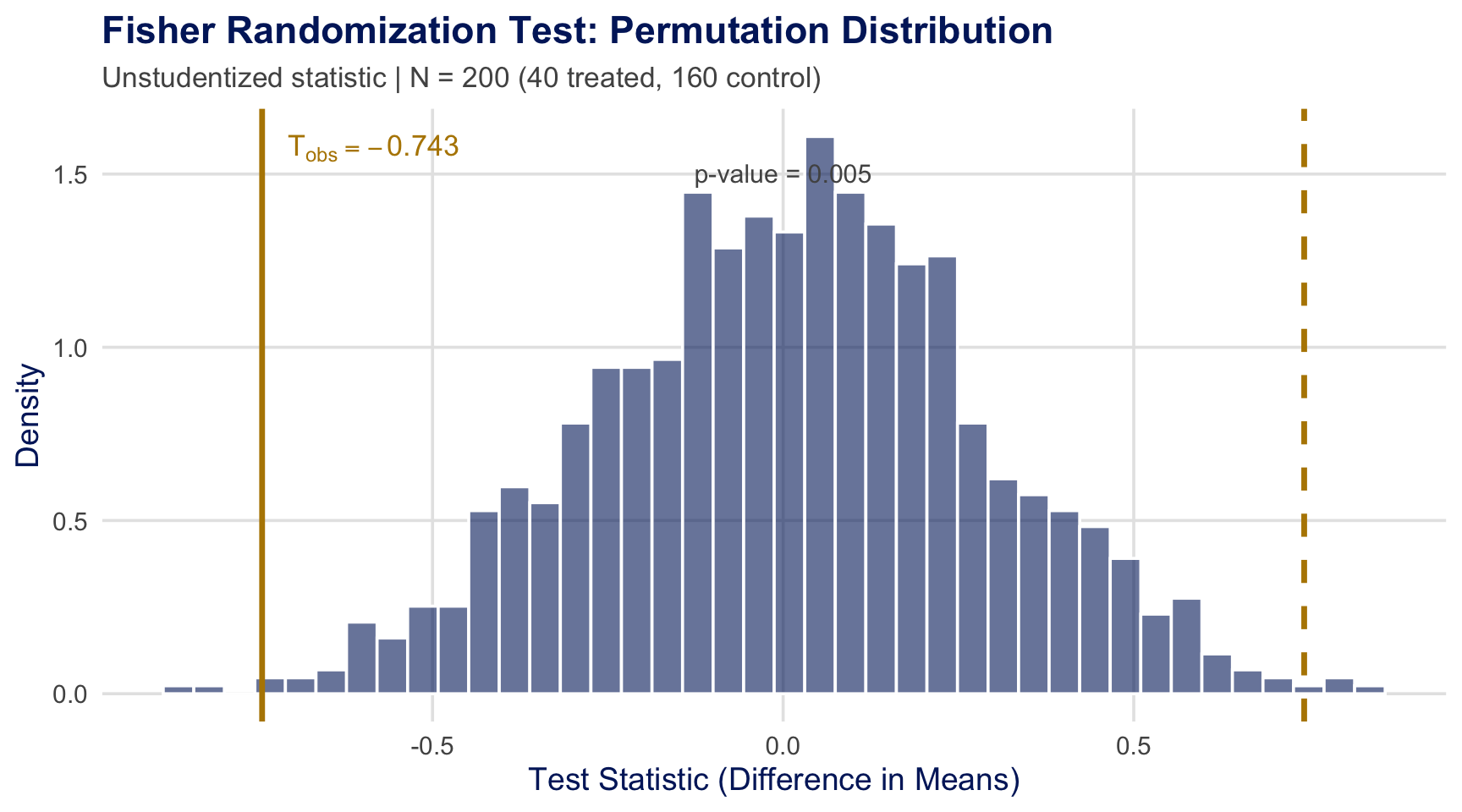
Visualizing Fisher Randomization Tests
- Illustration with simulated synthetic data
- Under the null, the observed assignment is “just another permutation”
- Procedure: (1) Compute \(T_{\text{obs}}\) from actual data \(\quad\) (2) Re-shuffle treatment \(\to\) recompute \(T^{\pi}\) \(\quad\) (3) \(p\text{-value} = \frac{\#\{|T^{\pi}| \geq |T_{\text{obs}}|\}}{B}\)
Why Studentization Matters
Simulation with synthetic data.
| Sharp null (\(H_0^S\)): \(Y_i(g) = Y_i(g')\) for all \(i, g, g'\) | \(\to\) FRT is exact |
| Weak null (\(H_0^W\)): \(\theta = 0\) | \(\to\) FRT may over-reject! |
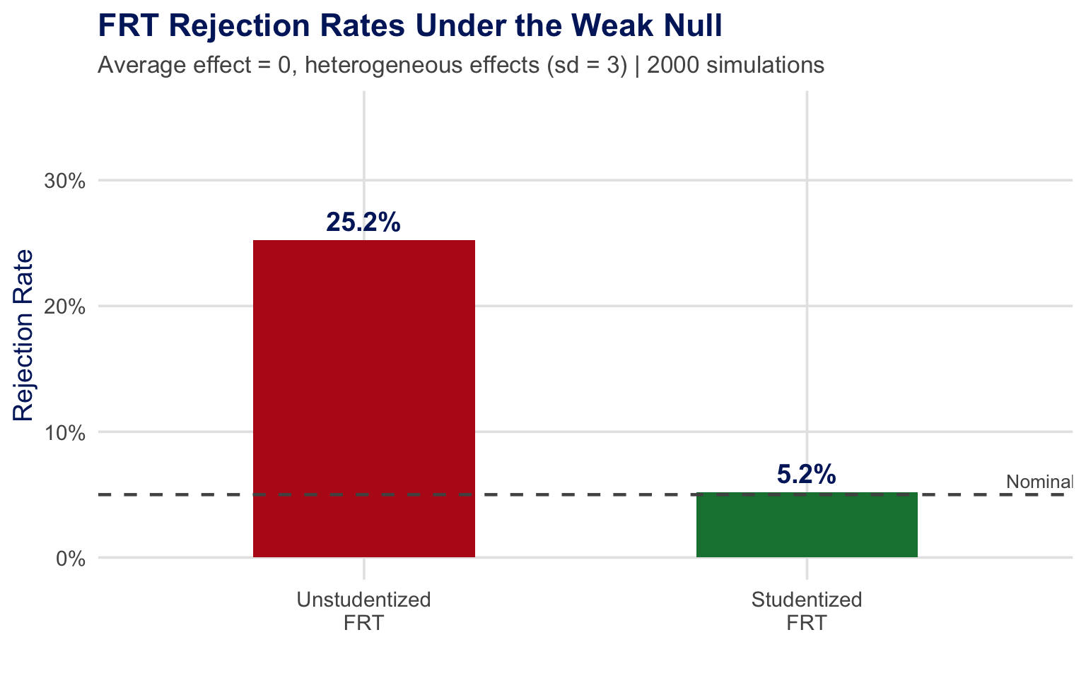
Under heterogeneous effects, unstudentized FRTs have severe size distortions. Studentization restores correct size (Wu and Ding 2021; Zhao and Ding 2021).
FRT for Callaway and Sant’Anna Estimators
- The randomization-based approach can also be applied to Callaway and Sant’Anna (2021) estimators
- Recall: CS is a special case with \(\beta = 1\)
- Thus, one can use FRTs to conduct “design-based” inference with CS estimators
- Rambachan and Roth (2025): FRT results are likely conservative even without full random timing — broadens applicability
Practical implication: Even if you use CS estimators (under weaker assumptions discussed in later lectures), you can supplement with FRT-based \(p\)-values when random timing is plausible. The staggered package implements this.
R Implementation
R Package: staggered
Installation: install.packages("staggered")
Main functions:
staggered(): Efficient estimator (Roth et al. 2023)staggered_cs(): Callaway and Sant’Anna (2021) estimatorstaggered_sa(): Sun and Abraham (2021) estimator
Built-in dataset: pj_officer_level_balanced (police training application)
Basic Usage: Efficient Estimator
Output: Returns estimate, se, se_neyman
Additional output: fisher_pval (permutation \(p\)-value)
Multiple Estimands
# Calendar-time weighted average
staggered(df = pj_officer_level_balanced,
          i = "uid", t = "period",
          g = "first_trained", y = "complaints",
          estimand = "calendar")

# Cohort-weighted average
staggered(..., estimand = "cohort")

# Event-study: effects at lags 0 through 11
staggered(df = pj_officer_level_balanced,
          i = "uid", t = "period",
          g = "first_trained", y = "complaints",
          estimand = "eventstudy",
          eventTime = 0:11)
Event-study returns one row per event time, each with its own estimate and SE.
Comparing Estimators
# Efficient estimator (Roth & Sant'Anna)
res_eff <- staggered(df = pj_officer_level_balanced,
    i = "uid", t = "period", g = "first_trained",
    y = "complaints", estimand = "simple")

# Callaway & Sant'Anna (2021)
res_cs <- staggered_cs(df = pj_officer_level_balanced,
    i = "uid", t = "period", g = "first_trained",
    y = "complaints", estimand = "simple")

# Sun & Abraham (2021)
res_sa <- staggered_sa(df = pj_officer_level_balanced,
    i = "uid", t = "period", g = "first_trained",
    y = "complaints", estimand = "simple")

# Unadjusted (no pre-treatment adjustment)
res_unadj <- staggered(df = pj_officer_level_balanced,
    i = "uid", t = "period", g = "first_trained",
    y = "complaints", estimand = "simple",
    beta = 1e-16, use_DiD_A0 = TRUE)
Application: Police Training Revisited
Application: Procedural Justice Training
- Setting: Wood, Tyler, and Papachristos (2020) — randomized rollout of procedural justice training to Chicago police officers
- Data: 5,537 officers, 72 monthly periods, 47 treatment cohorts (cohort sizes: 3–575)
- Outcomes:
- Complaints against officers
- Sustained complaints
- Officer use of force
- Treatment timing: Randomized by design \(\to\) random treatment timing holds
Comparison: Efficient estimator vs. Callaway-Sant’Anna vs. Sun-Abraham
Application Results: Complaints
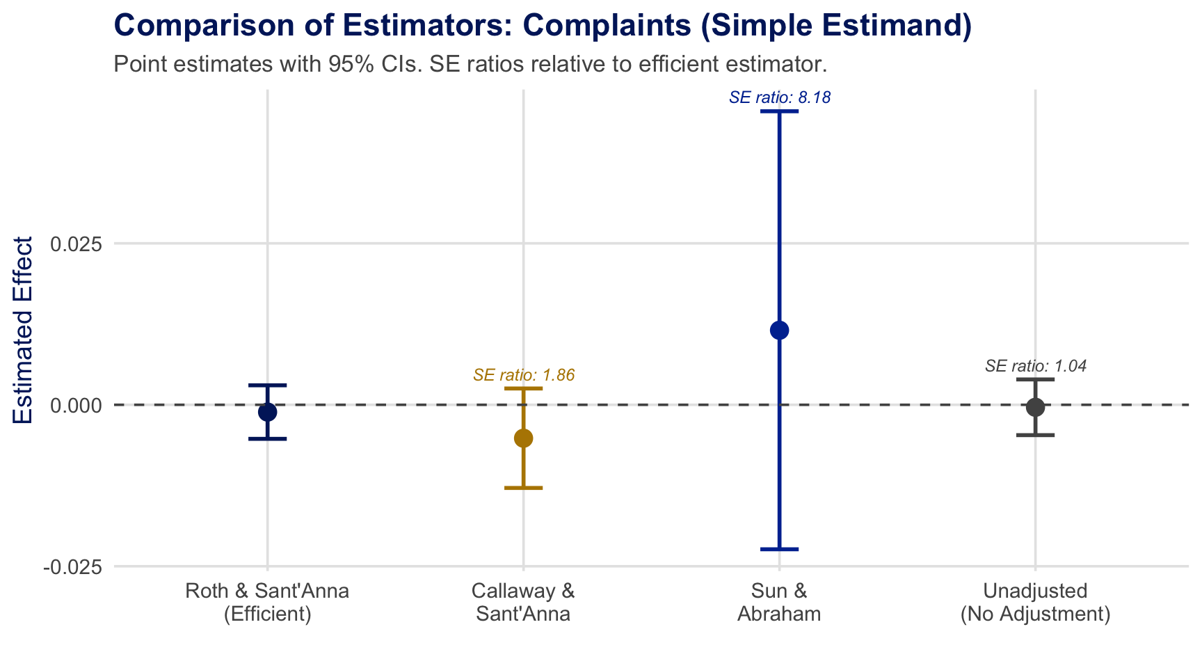
SE ratios annotated above each CI. Large gains over CS and SA; modest gains over unadjusted (\(\beta=0\)) — efficiency gains vary by application.
Application Results: Efficiency Gains Across Estimands
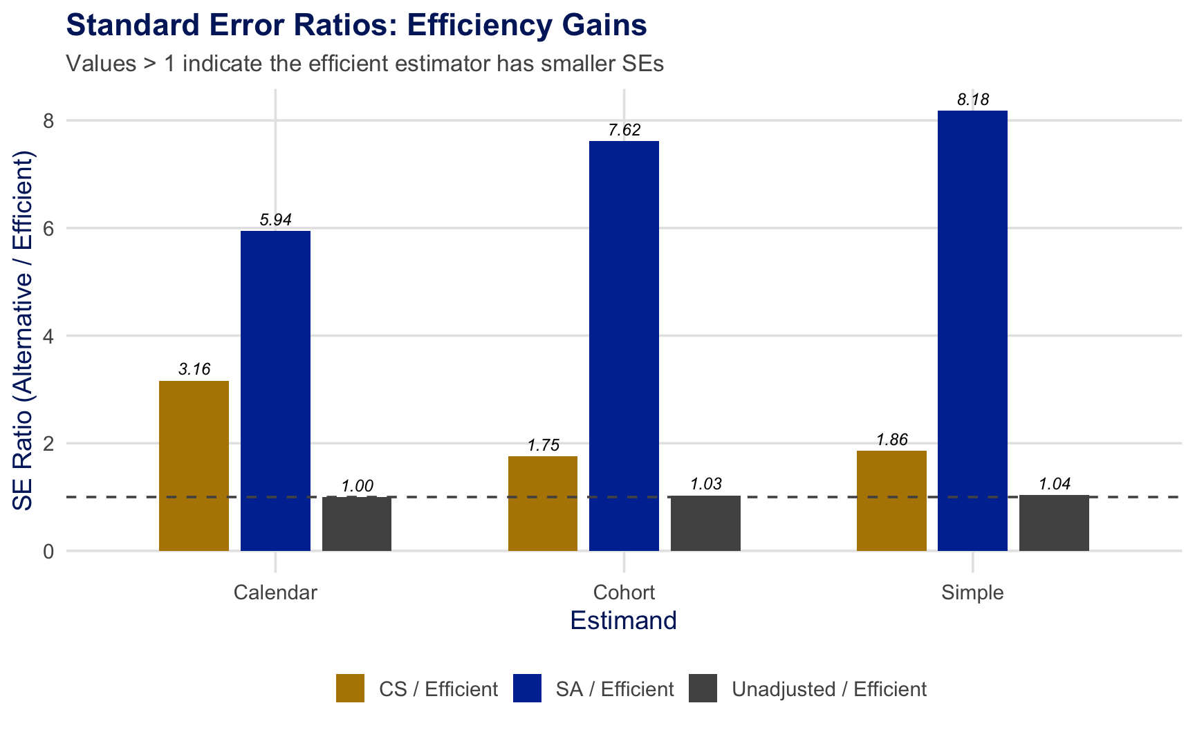
SE ratios \(>1\) indicate the efficient estimator has smaller standard errors.
Application Results: All Outcomes
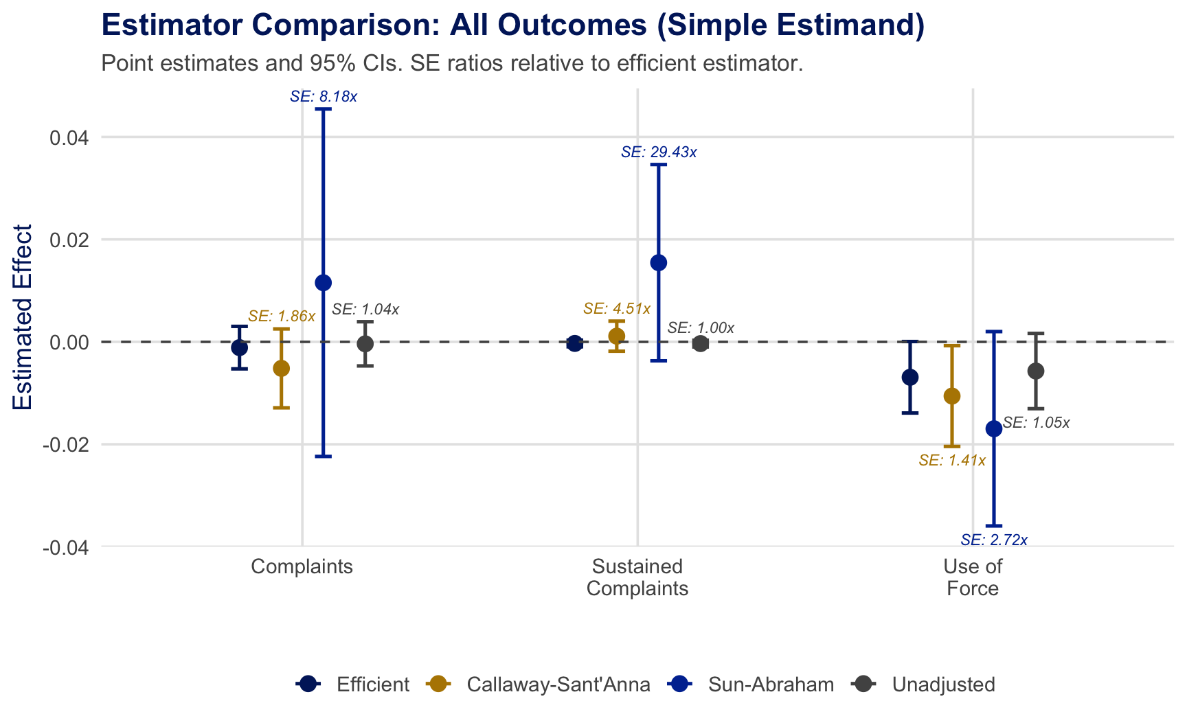
Efficiency gains vary across outcomes. Largest gains for sustained complaints; modest for use of force. SE ratios annotated above each CI.
Event Study: Complaints
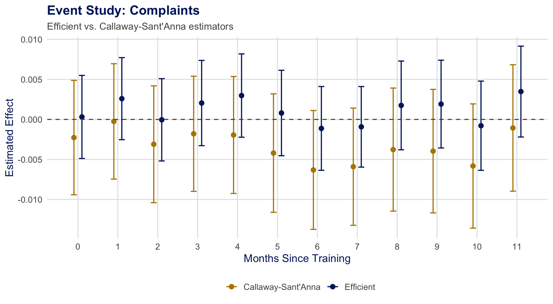
Efficient estimator (blue) produces tighter CIs at every event time, enabling sharper inference about dynamic treatment effects.
Can we assess the validity of the assumptions?
Balance Checks for Random Treatment Timing
- Under random treatment timing, pre-treatment outcomes should be balanced across cohorts
- Test \(H_0: \mathbb{E}[\hat{X}] = 0\) (pre-treatment differences are mean-zero)
- Roth et al. (2023): Propose balance checks implemented in
staggered
Results from police training data:
- Balanced on complaints and sustained complaints (main sample)
- Imbalanced when including pilot participants/special units (known to violate randomization)
- Pre-treatment event-study: no significant anticipation effects
Balance checks provide evidence for or against the random timing assumption — analogous to covariate balance checks in RCTs.
Take-Away
Take-Away Message
When treatment timing is random, estimators that use fixed adjustment weights (\(\beta = 0\) or \(\beta = 1\)) “leave money on the table”
Roth et al. (2023) show how to use additional information to “collect the money”
Estimators and inference easily implemented in R via the
staggeredpackageRecommendation: Use when treatment timing is (quasi-)random
- Other procedures remain valid under weaker assumptions (covered in upcoming lectures)
- Efficiency gains come from exploiting the additional structure of random timing
Next lecture: Observational panel data — when treatment timing is not random.
Summary of Key Results
| Result | Statement |
|---|---|
| Unbiasedness | \(\hat{\theta}_\beta\) is unbiased for \(\theta\) for any \(\beta\) (Lemma 2.1) |
| Efficiency | \(\beta^* = \text{Var}[\hat{X}]^{-1}\text{Cov}[\hat{X}, \hat{\theta}_0]\) minimizes variance (Prop. 2.1) |
| Feasibility | Plug-in \(\hat{\beta}^*\) achieves same asymptotic variance as oracle (Prop. 2.2) |
| Inference | Studentized FRT: exact under sharp null, valid under weak null (Prop. 2.3) |
| Nesting | \(\beta{=}0\), \(\beta{=}1\), CS, SA all special cases with fixed \(\beta\) |
| Gains | SE reductions of 1.4–8.4\(\times\) in application |
References
Appendix: Monte Carlo — Two-Period Design
DGP: Draw \(\mathbf{Y}_i(\infty) \sim \mathcal{N}(0, \Sigma_\rho)\); set \(Y_{i,2}(2) = Y_{i,2}(\infty) + \gamma(Y_{i,2}(\infty) - \mathbb{E}_{fin}[Y_{i,2}(\infty)])\)
- \(\gamma \in \{0, 0.5\}\): treatment effect heterogeneity; \(\rho \in \{0, 0.5, 0.99\}\): autocorrelation
- \(N_2 = N_\infty = N/2\), \(N \in \{25, 1000\}\)
Comparison: Plug-in efficient vs. full adjustment (\(\beta = 1\)) vs. no adjustment (\(\beta = 0\))
Key findings:
- All estimators unbiased; coverage \(\approx 95\%\)
- \(\rho = 0.99\): full adjustment optimal (\(\beta^* \approx 1\)); \(\rho = 0\): no adjustment optimal (\(\beta^* \approx 0\))
- Intermediate \(\rho\): plug-in can be 1.7\(\times\) more precise than full adjustment
Appendix: Monte Carlo — Staggered Design
Setup: Calibrated to police training data (72 periods, 48 cohorts, 7,785 officers). Sharp null: \(Y_{it}(g)\) = observed outcome for all \(g\).
Comparison: Plug-in efficient vs. Callaway-Sant’Anna vs. Sun-Abraham
Key findings:
- Plug-in: approximately unbiased, 93–96% coverage; FRT size \(\approx 5\%\)
- Efficiency gains vs. CS: SE ratio 1.39–1.85 (equivalent to 3.4\(\times\) the sample size)
- Efficiency gains vs. SA: SE ratio 3.0–6.86
Substantial efficiency gains are achievable in realistic staggered designs when treatment timing is random.
Appendix: FRT Simulation Code
Full Simulation Code: FRT Studentization
This simulation demonstrates why studentization is essential for FRTs under the weak null. Key DGP: heterogeneous treatment effects with unequal group sizes create variance asymmetry that the unstudentized FRT fails to account for.
set.seed(730)
N <- 200; n_treat <- 40; n_ctrl <- 160
n_perms <- 999; n_sims <- 2000; alpha <- 0.05
sigma_tau <- 3  # tau_i ~ N(0, sigma_tau^2), so E[tau]=0 (weak null)

# ---- Permutation Histogram (single simulation) ----
Y0 <- rnorm(N, 0, 1)
tau_i <- rnorm(N, 0, sigma_tau)
D <- c(rep(1, n_treat), rep(0, n_ctrl))
Y <- Y0 + D * tau_i
t_obs <- mean(Y[D == 1]) - mean(Y[D == 0])
t_perm <- replicate(n_perms, {
  D_p <- sample(D); mean(Y[D_p == 1]) - mean(Y[D_p == 0])
})

# ---- Rejection Rate Comparison (2000 simulations) ----
reject_unstud <- reject_stud <- 0
for (sim in 1:n_sims) {
  Y0 <- rnorm(N); tau_i <- rnorm(N, 0, sigma_tau)
  D <- c(rep(1, n_treat), rep(0, n_ctrl))
  Y <- Y0 + D * tau_i
  t_u <- mean(Y[D==1]) - mean(Y[D==0])
  se <- sqrt(var(Y[D==1])/n_treat + var(Y[D==0])/n_ctrl)
  t_s <- t_u / se
  t_perm_u <- t_perm_s <- numeric(n_perms)
  for (p in 1:n_perms) {
    Dp <- sample(D)
    Yt <- Y[Dp==1]; Yc <- Y[Dp==0]
    d <- mean(Yt) - mean(Yc)
    t_perm_u[p] <- d
    t_perm_s[p] <- d / sqrt(var(Yt)/sum(Dp) + var(Yc)/sum(1-Dp))
  }
  if (mean(abs(t_perm_u) >= abs(t_u)) < alpha) reject_unstud <- reject_unstud + 1
  if (mean(abs(t_perm_s) >= abs(t_s)) < alpha) reject_stud <- reject_stud + 1
}
cat("Unstudentized:", reject_unstud/n_sims,
    "| Studentized:", reject_stud/n_sims)
Application Figure Generation Code
Figures are generated from the pj_officer_level_balanced dataset in the staggered R package.
library(staggered)
data(pj_officer_level_balanced)
df <- pj_officer_level_balanced

# ---- Efficient vs. CS vs. SA vs. Unadjusted ----
res_eff <- staggered(df = df, i = "uid", t = "period",
  g = "first_trained", y = "complaints", estimand = "simple")
res_cs  <- staggered_cs(df = df, i = "uid", t = "period",
  g = "first_trained", y = "complaints", estimand = "simple")
res_sa  <- staggered_sa(df = df, i = "uid", t = "period",
  g = "first_trained", y = "complaints", estimand = "simple")

# ---- SE Ratios Across Estimands ----
for (est in c("simple", "calendar", "cohort")) {
  r_eff <- staggered(df=df, i="uid", t="period",
    g="first_trained", y="complaints", estimand=est)
  r_cs  <- staggered_cs(df=df, i="uid", t="period",
    g="first_trained", y="complaints", estimand=est)
  cat(est, ": CS/Eff SE ratio =", r_cs$se / r_eff$se, "\n")
}

# ---- Event Study ----
es_eff <- staggered(df=df, i="uid", t="period",
  g="first_trained", y="complaints",
  estimand="eventstudy", eventTime=0:11)
es_cs <- staggered_cs(df=df, i="uid", t="period",
  g="first_trained", y="complaints",
  estimand="eventstudy", eventTime=0:11)

# See Figures/Lecture4/generate_figures.R for full code
ECON 730 | Causal Panel Data | Pedro H. C. Sant’Anna