DiD Resources
I have collected links to several resources on this webpage to make Difference-in-Differences (DiD) materials even more accessible to the community.
I will update and add to these materials as time passes. So please keep an eye on this webpage!
I prepared this slide deck to present at NABE TEC 2024 in Seattle in October 2024. It introduces DiD to a broader audience and outlines the problems and solutions associated with staggered treatment adoption.
This is the slide deck I have prepared to present at Instacart in September 2024. It overviews the basics of DiD, discusses a DML DiD implementation that leverages covariates, and then discusses staggered adoption.
I prepared this slide deck for a guest lecture at USP in Brazil in November 2022. It summarizes the "big course" into a two-hour lecture.
I have assembled these 14 slide decks to help more people start or deepen their journey through DiD methods. These slides are inspired by my 30-to-40 hours DiD course at Causal Solutions.
[Summary] [Slides]
We introduce DiD, discuss its popularity in economics, present several examples of DiD applications, and discuss the importance of using the appropriate potential outcome notation to define the causal parameter of interest.
[Summary] [Slides]
We discuss the two-group-two-periods DiD setup in great detail. We pay particular attention to the identifying assumptions and derive the large sample properties of canonical DiD estimators. We also discuss clustering and the multiplier bootstrap.
[Summary] [Slides]
We discuss the challenges when there are not many clusters available. In particular, we discuss different approaches to conducting inference in this challenging setup, highlighting that these alternative inference procedures often implicitly add restrictions on treatment effect heterogeneity. No perfect solution seems to exist here, though, and one should be aware of the trade-offs.
[Summary] [Slides]
We highlight that parallel trends may have different interpretations depending on how you measure your outcome (e.g., level or log). We discuss the results in Roth and Sant'Anna (2023, ECMA) that characterize when parallel trends is sensitive to functional form, and how one can test for these conditions. We end the slide pointing out that you can easily use our proposed test using the
R package didFF .
[Summary] [Slides]
We introduce the conditional parallel trends assumption and highlight that this assumption allows for covariate-specific trends. We then show that traditional TWFE regression specifications that include covariates linearly do not respect conditional parallel trends and, therefore, can lead to biased ATT estimates. We then discuss three more reliable estimation strategies based on regression adjustment (outcome regression), inverse probability weighting, and doubly robust methods. We illustrate these estimators' appeal and flexibility via Monte Carlo simulations.
All these more appropriate estimators are easy to use via the R packages
DRDID and
did, the Stata packages
drdid,
csdid, and
csdid2, and the Python packages
drdid, and
csdid.
[Summary] [Slides]
We discuss how one can leverage the doubly robust DiD formulation to estimate the ATT using modern machine-learning estimators for the nuisance functions. The slides discuss LASSO in more detail. For the case of LASSO, under appropriate conditions, it suffices to run LASSO for the outcome regression and the propensity score, collect all the ``selected'' covariates, and use them as if we knew these were the only relevant covariates for the DiD (so this is a post-LASSO DR DiD estimator). Of course, you can also use other ML estimators, but more tuning is needed for those cases.
[Summary] [Slides]
Although DiD can be used with panel or repeated cross-sectional data, there are important differences between these two sampling schemes. In this lecture, we discuss some of these differences and highlight that most available DiD procedures that leverage repeated cross-sections (RCS) rule out compositional changes over time, a type of stationarity assumption. We point readers to recent work that discusses tests for this stationarity condition and the importance of modeling outcome evolution among treated and untreated units when only RCS is available. We also discuss the loss of efficiency associated with not having access to balanced panel data.
[Summary] [Slides]
We discuss setups where one can access data from several periods, allowing them to learn how treatment effects evolve over elapsed treatment time, often referred to as an event study. We talk about parameters of interest, an appropriate notion of parallel trends, and how to identify, estimate, and make (uniformly valid) inferences about the ATT at different points in time. We discuss the DiD setups with and without covariates.
One can implement the discussed event-study estimators using the
did R package, the Stata packages
csdid and
csdid2, and the Python package
csdid.
[Summary] [Slides]
We discuss the treatment effect parameters one recovers using static, dynamic, and semi-dynamic TWFE specifications without covariates in DiD setups with multiple periods (but a single treatment date). We highlight that one needs to strengthen the parallel trends assumption and adjust the estimation procedure accordingly to leverage all the information from pre-treatment periods to get more precise post-treatment DiD estimates.
[Summary] [Slides]
We discuss how to explore pre-treatment data to assess the plausibility of the identifying assumptions in DiD. We also discuss that pre-tests based on pre-treatment data are neither necessary nor sufficient for (some versions of) parallel trends. We also discuss how the no-anticipation and parallel trends interact.
Although this lecture does not cover issues related to power and how to conduct sensitivity analysis for violations of PT, I strongly recommend you to take a look at
these slides by Jon Roth. [Summary] [Slides]
We discuss the pitfalls of using standard TWFE regression specifications to estimate average treatment effects in DiD setups with variations in treatment timing. These slides highlight that standard TWFE specifications have several drawbacks, including aggregating treatment effects using negative and non-interpretable weights. We cover the Bacon-Decomposition of Goodman-Bacon (2021, JoE), the dCDH decomposition of de Chaisemartin and D’Haultfoeuille (2020, AER) decomposition, and the negative event-study results of Sun and Abraham (2021, JoE). This slide deck suggests that empirical researchers should be very careful when using TWFE in setups with variations in treatment timing. Personally, I recommend not even bothering with it.
[Summary] [Slides]
I usually call the negative results of TWFE in the previous slide the ``Sad results", as these just point out problems, making our lives harder. In sharp contrast, I call the results that show how one can completely avoid those problems using simple and intuitive strategies the ``Happy results/papers''. I am all about ``happy papers,'' and this lecture covers precisely that: how one can bypass the (artificial) challenges associated with TWFE and get reliable estimators that respect your identification assumptions. I discuss in great detail how one can use the DiD estimators proposed by Callaway and Sant'Anna (2021, JoE) to ``estimate yourself out'' of the TWFE hell. I also briefly discuss other estimators that share the same philosophy as Callaway and Sant'Anna (2021): one should separate identification, aggregation, and estimation/inference steps in staggered DiD.
One can implement the discussed CS estimators using the
did R package, the Stata packages
csdid and
csdid2, and the Python package
csdid.
[Summary] [Slides]
Sometimes, treatments turn on-and-off over time. This lecture discusses the challenges associated with this setup when using DiD-type strategies. We index the potential outcomes with treatment sequences and discuss the different causal parameters of interest in this more complex setup. As the number of parameters here tends to be very large, one may wish to aggregate them further to gain some precision. We discuss this and highlight that absent additional assumption that limit treatment effect heterogeneity/dynamics; it is hard to interpret these parameters.
[Summary] [Slides]
We discuss setups where treatment timing is as-good-as-random, as in Roth and Sant'Anna (2023, JPE: Micro). We highlight that in such cases, it is possible to form alternative estimators that more efficiently leverage the random treatment timing assumption and produce substantially more precise estimators than popular staggered DiD estimators. We discuss how one can conduct randomization-based inference procedures in this setup. We also illustrate the appeal of the proposed tools in an application that studied a randomized rollout of a procedural justice training program for police officers.
One can implement the more efficient staggered estimators using the
R package staggered, and the
Stata package staggered .
- Triple Differences
- DiD with Continuous Treatment
- Instrumented DiD
- Synthetic DiD and related extensions
- Heterogeneity analysis in DiD
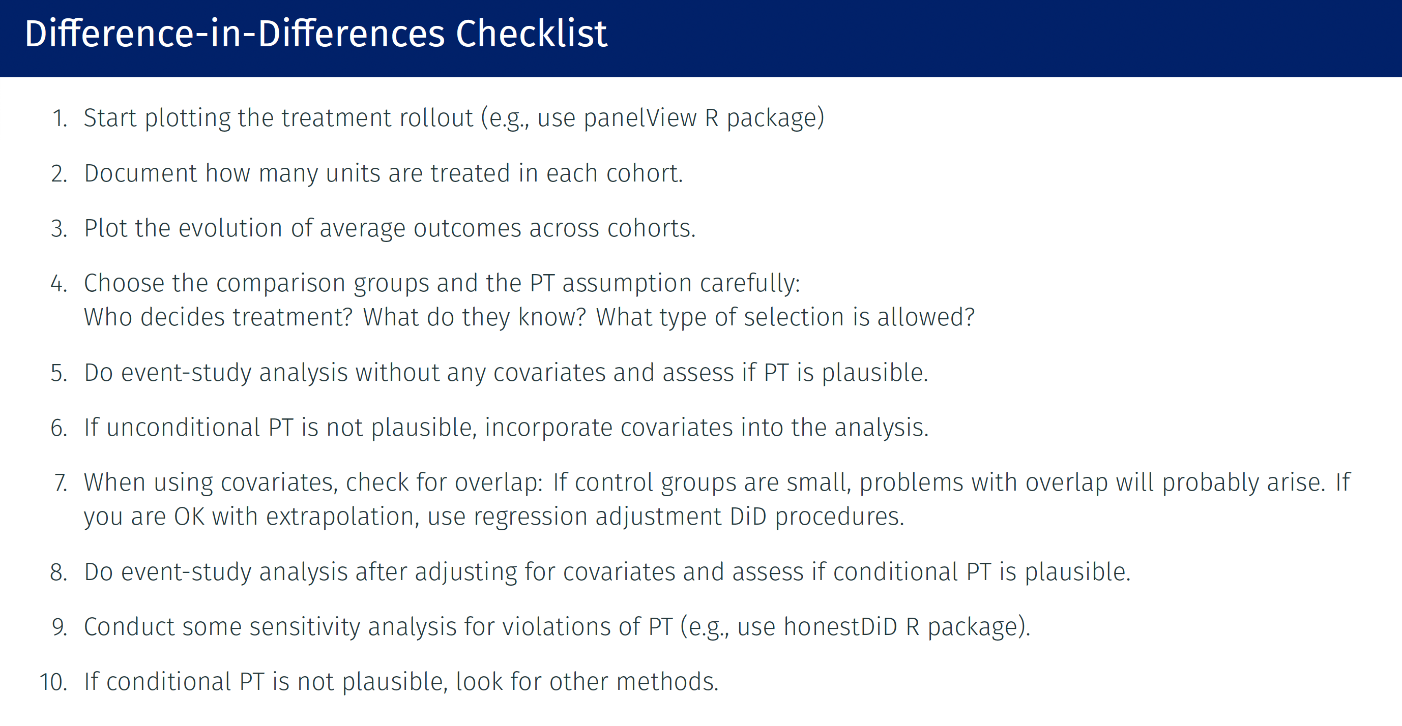
Over the years, many people have asked me for advice on best practices for conducting their DiD analysis. I created the following checklist to provide a first-order approximation of these questions. Please do not take it literally. It is meant to be interpreted more as an informal guide than a protocol.

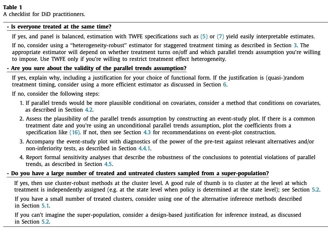
If you are interested in a succinct overview of the (by then) recent DiD literature, see my Journal of Econometrics paper, “What’s trending in difference-in-differences? A synthesis of the recent econometrics literature”. Over there, we provided a checklist for practitioners that you may find helpful.

I have co-created several DiD packages, as I describe below:
Implements a variety of DiD estimators in setups that potentially have multiple periods, staggered treatment adoption, and when parallel trends may only be plausible after conditioning on covariates. Based on Callaway and Sant'Anna (2021).
[R package] [Stata package] [Python package]
Implements 2x2 DiD estimators in setups where the parallel trends assumption holds after conditioning on a vector of pre-treatment covariates. Based on Sant'Anna and Zhao (2020).
[R package] [Stata package] [Python package]
Implements the efficient estimator for settings with (quasi-)random treatment timing proposed in Roth and Sant'Anna (2023, JPE: Micro). It also implements the design-based versions of Callaway & Sant'Anna and Sun & Abraham estimators (without covariates).
[R package] [Stata package]
Implementes a test for whether parallel trends is insensitive to functional form by estimating the implied density of potential outcomes under the null and checking if it is significantly below zero at some point. Based on Roth and Sant'Anna (2023, ECMA).
[R package]
Here are some additional materials developed by some of my friends that cover topics that I have not covered in my lectures:
[Introduction] [Relaxing Parallel Trends] [More Complicated Treatment Regimes] [Alternative Identification Strategies]
[Introduction] [Staggered Treatment Timing] [Violations of Parallel Trends]


